How to construct Atom Centered Symmetry Functions (ACSFs)
In chemistry, the most common way of representing molecules is to use Cartesian coordinates.

The problem of Cartesian coordinates is that if one rotates or translates a molecule, the coordinates change. However, properties like the total energy of the molecule, the dipole moment or the atomisation energy remain unchanged.
Therefore, if you want to learn the properties of a molecule with a machine learning algorithm like neural networks, you want to represent the molecular structure in a way that doesn’t change when you rotate or translate the molecule.
By doing this, you make the training process more efficient because the neural network doesn’t need to learn that many different Cartesian coordinates represent the same structure.
This is where Atom Centred Symmetry Functions (ACSF) come in handy. They are a way of representing a molecular structure which remains the same when the molecule is rotated or translated.
How do they work
Two-body term
Note: in this post I will use the functional form of ACSF described by Smith et al. in this publication.
ACSF generally include two and three-body terms. For example, the two body term is usually written in papers as:
\[S_i(radial) = \sum_{j \neq i \\ Z_j = Z} e^{-\eta (R_{ij} - R_s)} f_c(R_{ij}, R_c)\]This can be quite confusing, so let’s break it down. The sum is over atoms \(j\), which are the neighbours of atom \(i\) atom type \(Z\). \(\eta\) and \(R_s\) are parameters that are picked by the user. \(R_{ij}\) is the distance between atom \(i\) and \(j\). The last term \(f_c(R_{ij})\) is a cut off function which depends on the distance between the atoms and on a cut-off distance \(R_c\).
If you are worried about the sum over neighbours of a particular atom type, rest assured. We shall go through it with examples.
Let’s say that we have a toy-system with 5 particles, of 3 different types.
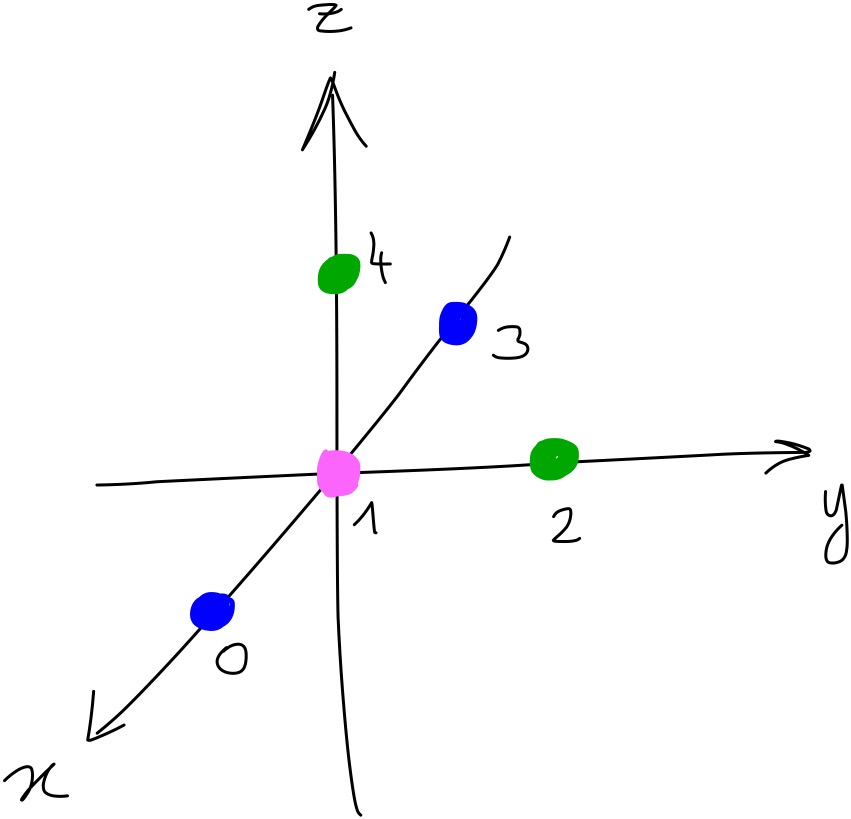
The snippet below shows the coordinates of all the particles and their type. Blue particles are of ‘type 0’, pink particles are of ‘type 1’ and green particles are of ‘type 2’. Below are the coordinates of the particles in the toy system as they would be in a Python script:
import numpy as np

xyz = np.array([[1, 0, 0],
                [0, 0, 0],
                [0, 1, 0],
                [-1, 0, 0],
                [0, 0, 1]])

types = np.array([0, 1, 2, 0, 2])
If we want to calculate the two-body term for particle 0, we construct it as follows. We make a vector where for each element \(S_0^{(t)}\)the sum is over particles of type \(t\). This can be shown with an image:

For \(S_0^{(0)}\) the sum is over blue particles, for \(S_0^{(1)}\) it is over pink particles and for \(S_0^{(2)}\) it is over green particles. With some code, where r_i represents the coordinates of particle i and where \(\eta = 1\), \(R_s = 0\) and \(R_c = 5\):
def f_c(r_ij, r_c):
    """
    This is the cut-off term
    :param r_ij: distance between atom i and j
    :param r_c: cut off distance
    """
    if r_ij < r_c:
            f_c = 0.5 * (np.cos(np.pi * r_ij / r_c) + 1.0)
    else:
            f_c = 0.0
    return f_c

r_s = 0
r_c = 5
eta = 1

s_0 = np.zeros(3)

s_0[0] = np.exp(-eta*(r_3 - r_s)**2) * f_c(r_3, r_c)
s_0[1] = np.exp(-eta*(r_1 - r_s)**2) * f_c(r_1, r_c)
s_0[2] = np.exp(-eta*(r_2 - r_s)**2) * f_c(r_2, r_c) + np.exp(-eta*(r_4 - r_s)**2) * f_c(r_4, r_c)
This gives s_0 = [0.01198774, 0.33275008, 0.22066655]. Now, let’s do the same for particle 1. Again, we make a vector where for each element \(S_1^{(t)}\) the sum is over particles of type \(t\).
s_1 = np.zeros(3)

s_1[0] = np.exp(-eta*(r_10 - r_s)**2) * f_c(r_10, r_c) + np.exp(-eta*(r_13 - r_s)**2) * f_c(r_13, r_c)
s_1[1] = 0
s_1[2] = np.exp(-eta*(r_12 - r_s)**2) * f_c(r_12, r_c) + np.exp(-eta*(r_14 - r_s)**2) * f_c(r_14, r_c)
As you can see, now \(S_1^{(0)}\) has two terms in the sum. This is because particle 1 (in pink) is close to two blue particles. However, it doesn’t have any pink neighbours, so \(S_1^{(1)}\) remains zero. This results in \(S_1\) being [0.66550016, 0.0, 0.66550016].
This process is then repeated for each particle in the system, so you end up with 5 vectors of length 3.
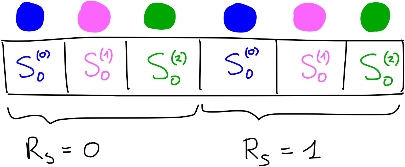
There is one final step that needs to be done to have the complete two-body term. Remember the parameter \(R_s\)? Usually you don’t use only one value of \(R_s\), but many. You need to repeat the calculations we have done above, but with a different value of \(R_s\), for example \(R_s = 1\). Then, you concatenate the new vector of length 3 to the one obtained with \(R_s = 0\).
For example, for particle 0, if we used \(R_s = 1\) we would obtain the values [0.24078022, 0.9045085, 1.37344827] for \(S_0\). By combining these with the ones obtained above using \(R_s = 0\), the full \(S_0\) two-body term would be [0.01198774, 0.33275008, 0.22066655, 0.24078022, 0.9045085, 1.37344827]. With an image:
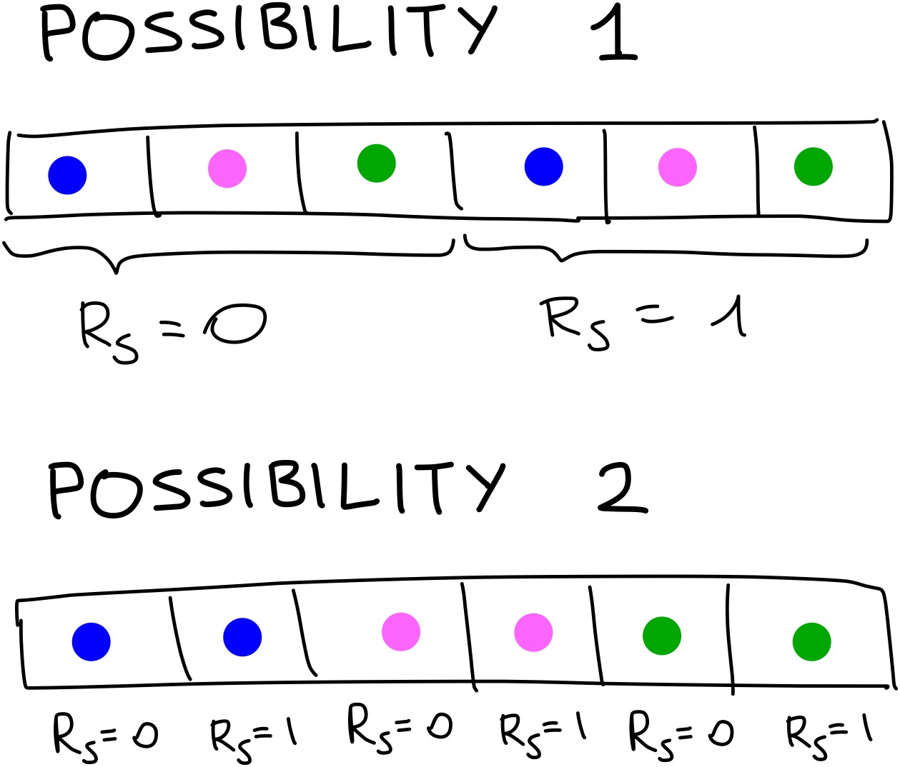
One minor point to note is that it doesn’t matter in which order you concatenate the vectors. You could calculate all the terms for particle 0 interacting with a blue particle with different values of \(R_s\), then have a vector with all the interactions with pink particles with the different values of \(R_s\) and finally all the interactions with green particles. This again is more easily shown with an image:
Three-body term
If you have made it this far, well done! The most complicated part is now over. The principle is the same for the three body term, except that there are more parameters and we look at 2 neighbours at a time!
The three body term is expressed as:
\[S_i(angular) = 2^{\zeta -1} \sum_{j \neq i, j \neq k} (1 + \cos(\theta_{ijk} - \theta_s))^\zeta \times e^{-\eta \frac{R_{ij} + R_{ik}}{2} - R_s} f_c(R_{ij}, R_c) f_c(R_{ik}, R_c)\]The parameters that need to be picked by the user are: \(\zeta\), \(\eta\), \(\theta_s\) and \(R_s\). Remember how in the two body term the parameter \(R_s\) took multiple values? Here both \(R_s\) and \(\theta_s\) take multiple values. The only other variable that hasn’t been introduced yet is \(\theta_{ijk}\), which is the angle between particles \(i\), \(j\) and \(k\).
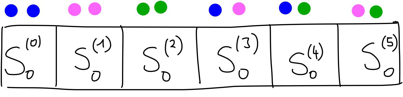
Now, let’s construct the three body term for particle zero. The sum in \(S_i(angular)\) is over pairs of neighbour types. The possible pairs of neighbour types are:
[00, 11, 22, 01, 02, 12]
where the order of the pairs doesn’t matter - i.e. 01 = 10. So, the first part of the three body term for particle 0 \(S_0(angular)\) can be visualised as follows:
And expressed with some code (the values of the parameters r_s, theta_s, … are included in the function for readability):
def s_ang_term(r_ij, r_ik, theta_ijk)
    """
    This calculates the angular term for a particular atom and 2 of its neighbours.
    :param r_ij: the distance between atom i and j
    :param r_ik: the distance between atom i and k
    :param theta_ijk: the angle between atom i, j and k
    """
    r_s = 0
    theta_s = 0
    eta = 1
    zeta = 1
    r_c = 5
    term = (1 + np.cos(theta_ijk - theta_s))**zeta * np.exp((0.5*(r_ij + r_ik) - r_s)**2) * f_c(r_ij, r_c) * f_c(r_ik, r_c)

    return term * 2**(1-zeta)

S_0_ang = np.zeros(6)

S_0_ang[0] = 0
S_0_ang[1] = 0
S_0_ang[2] = s_ang_term(r_02, r_04, theta_024)
S_0_ang[3] = s_ang_term(r_01, r_03, theta_013)
S_0_ang[4] = s_ang_term(r_02, r_03, theta_023) + s_ang_term(r_03, r_04, theta_034)
S_0_ang[5] = s_ang_term(r_01, r_02, theta_012) + s_ang_term(r_01, r_04, theta_014)
The first two terms are zero because there are no two other blue particles or two pink particles near particle 0. The third term captures the interaction of particle 0 with particle 2 and particle 4 which are both green.
Now, this process has to be repeated with different values of \(R_s\) and \(theta_s\). For example, if we chose to use \(R_s = [0, 1]\) and \(\theta_s = [0, \pi]\), then, we would end up with four vectors of length 6 to be concatenated. This can be shown with an image:
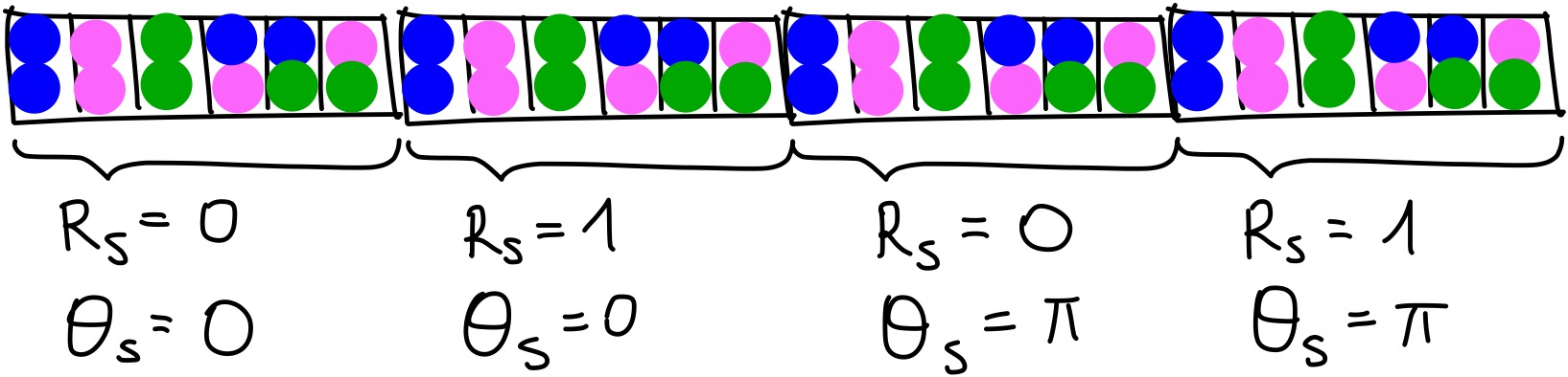
And then repeat this process for every particle!
Once all the 2 and 3-body terms are obtained for each particle, they are also concatenated. In this way, you have 1 vector for each particle.
If you are interested in an implementation that is easy to understand, I have made one in Numpy that you can find here. This implementation is very slow, so don’t use it if you have many values of the parameters or many molecules. If you want a faster implementation, you can have a look at this one. It is implemented in TensorFlow, so it is harder to read, but it is much faster.
That implementation is part of the python package QML (Quantum Machine Learning), which can be used to generate a variety of descriptors and then use them for either Kernel Ridge Regression or Neural Networks.